Randomness
In this post I will start exploring the basics of randomness and related functionality in APL. I want to eventually get to a point where I am doing MCMC for some data implemented from scratch.
Since I do not have any experience with APL, I am at a point where I basically know what I want to do, but not exactly how, I will also post docs outputs and my reactions to them. These basic steps are left in so the reader (likely myself in the future) will recall how the actual workflow of using dyalog goes.
The basics
In APL the symbol that is associated with randomness is ?.
In APL the docs are generally pretty helpful, however when using it on a symbol, we get a link:
]HELP ?https://help.dyalog.com/19.0/Content/Language/Symbols/Question%20Mark.htm
Following the link leads us to the below content.
Monadic Question Mark means
Roll

      ? 6 6 6 6 6
4 3 6 3 5

      ? 0 0
0.260561 0.929928
Dyadic Question Mark means
Deal

      13 ? 52
36 31 44 11 27 42 13 8 2 33 19 34 6
Language Elements
Monadic use
Above, we can see the word "Monadic" mentioned.
"Monadic" means that when used with a single argument after the symbol, like ? 1 2 3 4, then we will get some random numbers.
? 1 2 3 41 1 1 3
There are basically two modes of execution for the Roll function.
The function can only be used with a non-negative integer.
If used with 0, then it rolls a number betweenn 0 and 1.
If used with a positive integer \(N\), then it will roll a \(N\) -sided die.
If rolled with \( N=1 \), it rolls a 1-sided die that always lands on 1.
Also, for the inexperienced APL reader (yours truly) it might look like we are passing multiple arguments to the ? function. However multiple numbers delimited by spaces in dyalog are actually a vector so we are passing a single vector argument.
? 00.8470255226
(Short Excursion:) Plotting in APL
Since the docs didn't really line out the above very clearly, I basically had to "confirm" for myself that what I said is true. To do that more effectively I wanted to plot numbers.
After a bit of searching on the internet, I have found that plotting is very easy. Like this:
]plot {1○(⍳⍵)×○4÷⍵}2000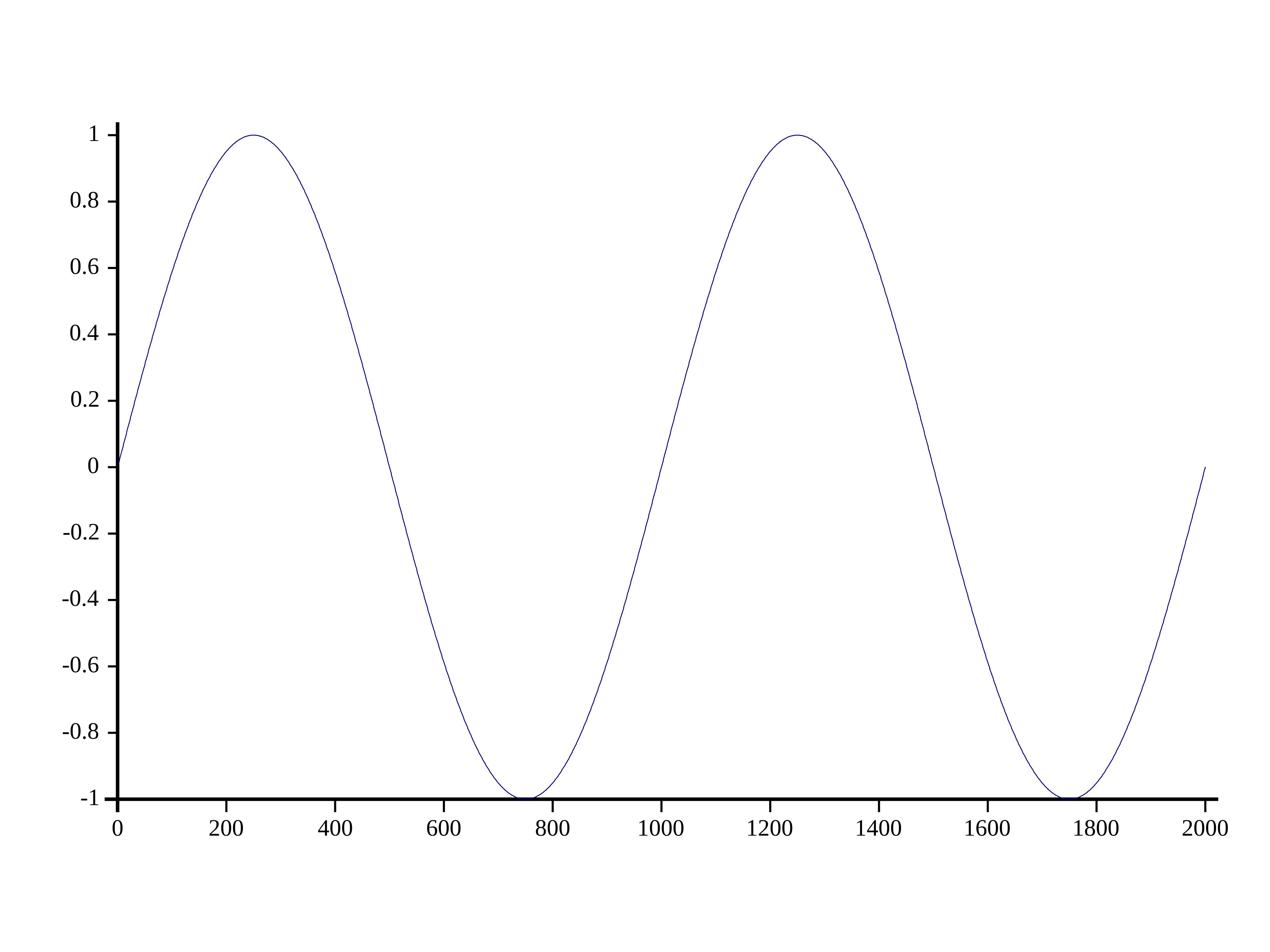
If we give it a vector, then it will just plot all those number on the y axis, and the x-axis will be the indices of the numbers.
⍴ {1○(⍳⍵)×○4÷⍵}20002000
When we pass a second vector as input, they will be the x values Very easy to see like this.
]plot (1 2 4 8 16) (1 2 3 2 5)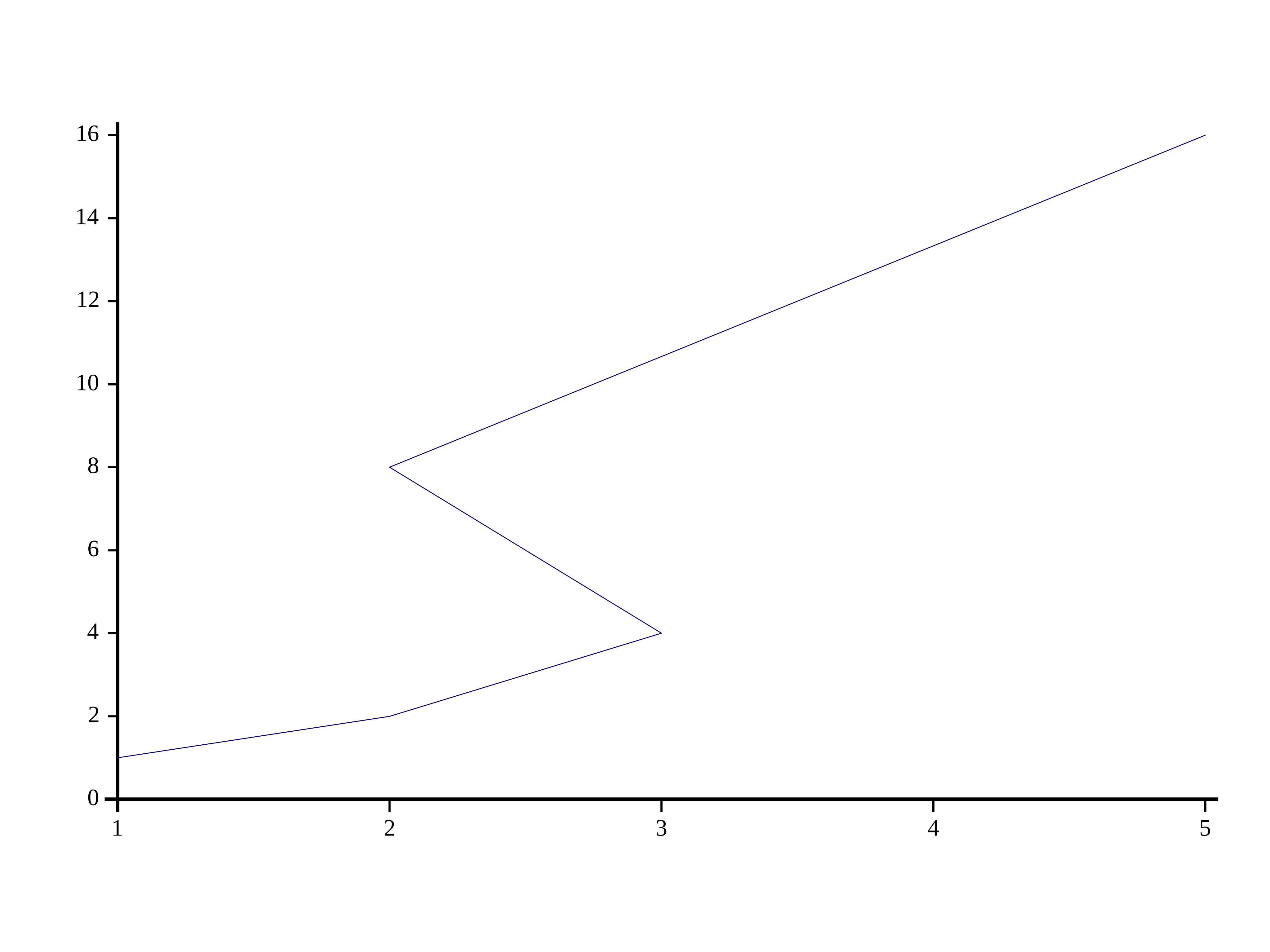
Lets have a look at the docs of the ]plot functionality, since I really wanna just make a simple histogram, but don't wanna do the binning myself.
]plot -???
───────────────────────────────────────────────────────────────────────────────

]OUTPUT.Plot

Plot data
    ]Plot <data> [-type=<name>]

<data>  a simple vector or a vector of vectors (one per co-ordinate or series)
<name>  the type of chart to be produced (default: Line), one of:
      Bar         side-by-side bars rising from a baseline
      Box         quartiles of mono- or bi-variate numerical distributions
      Bubble      bubbles scaled by Z value at XY positions
      Cloud       markers on a 3D XYZ space
      Contour     2D projection of XYZ regression surface
      Dial        arrows pointing at values on a semi-circular dial
      Gantt       bars, specifying start and end points
      Histogram   the value distribution of an unordered series
      Line        connected values on an XY plane
      MinMax      mono-variate ranges on an XY plane
      Pie         numeric series as angular portions of a disk
      Polar       XY series where X is angular
      Response    Z surface on a 3D XYZ space
      Scatter     markers on an XY plane
      Step        a constant XY line with discrete changes
      Table       rows and columns of text
      Tower       a matrix of Z-scaled bars on a 3D XYZ space
      Trace       XY lines alongside
      TreeMap     nested rectangles of specified area (and possibly altitude)
      Triangle    proportions of 3 variables on a triangle
      Vector      XY vectors
      XBar        bars at specified X positions

Rendering will happen by sending through the RIDE protocol if APL is being controlled through that (as is the case right now), otherwise a stand-alone HTMLRenderer will be used.
Ok it seems as though you can make a histogram by putting -type=Hist after ]plot. Thats quite convenient.
Next, lets look at the distribution of the random numbers, to know how we have to write random matrices / vectors.
We know that we can make empty arrays with ⍴.
2 3 ⍴ 00 0 0 0 0 0
So we can make 200 random numbers like this:
? 20 ⍴ 00.7468686341 0.5853161536 0.01495771382 0.5840063831 0.1730637546 0.3003460386 0.3480738525 0.4596478788 0.7069295596 0.7251053055 0.3505076734 0.9459180567 0.3710854316 0.8108662854 0.09304922758 0.09956130643 0.6459058321 0.8849648041 0.9015517188 0.6587623089
]plot -type=Histogram (? 2000 ⍴ 0)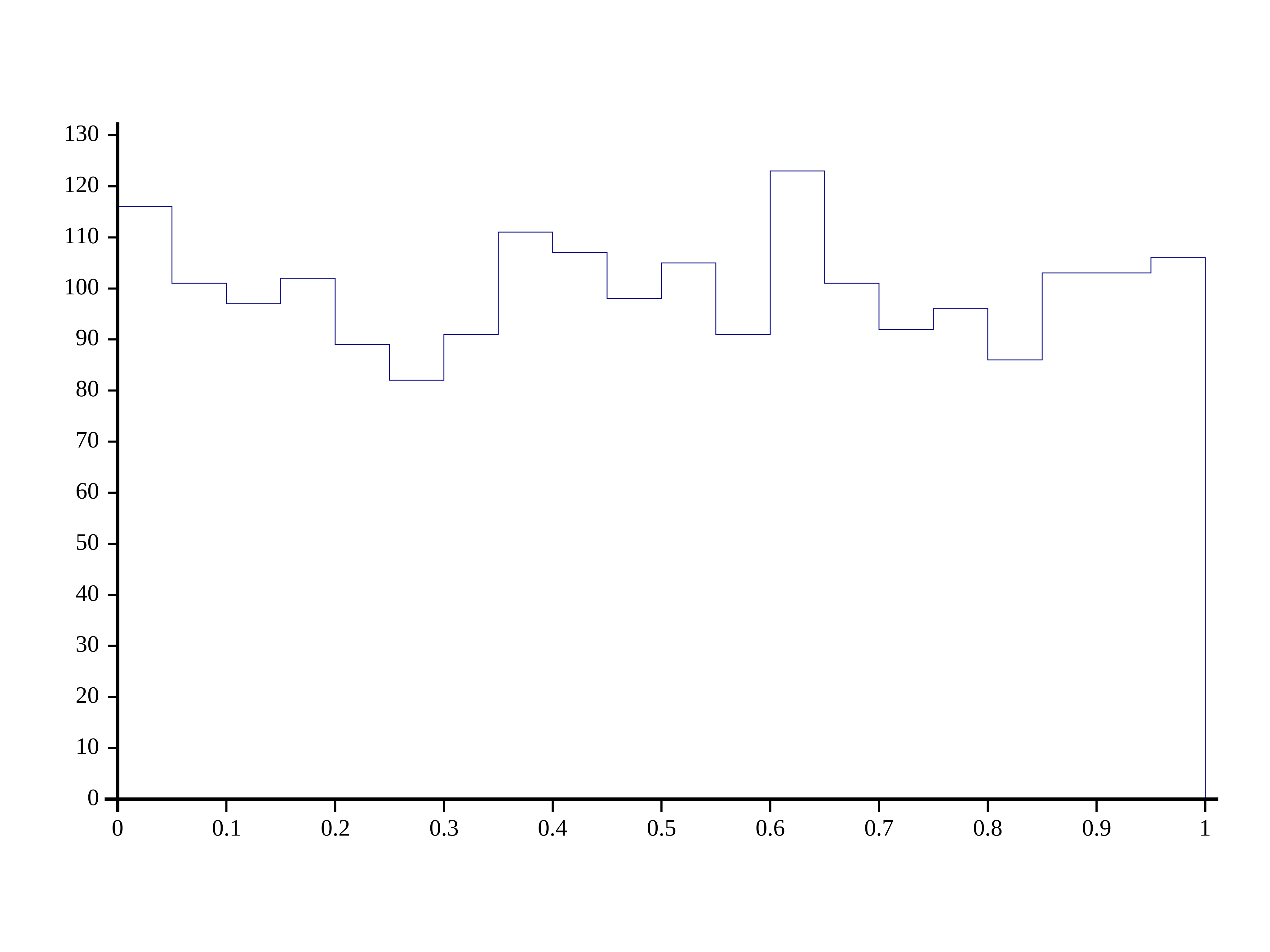
Yeah it seems to be a uniform distribution between 0 and 1 if the argument is 0.
]plot -type=Histogram (? 2000 ⍴ 1)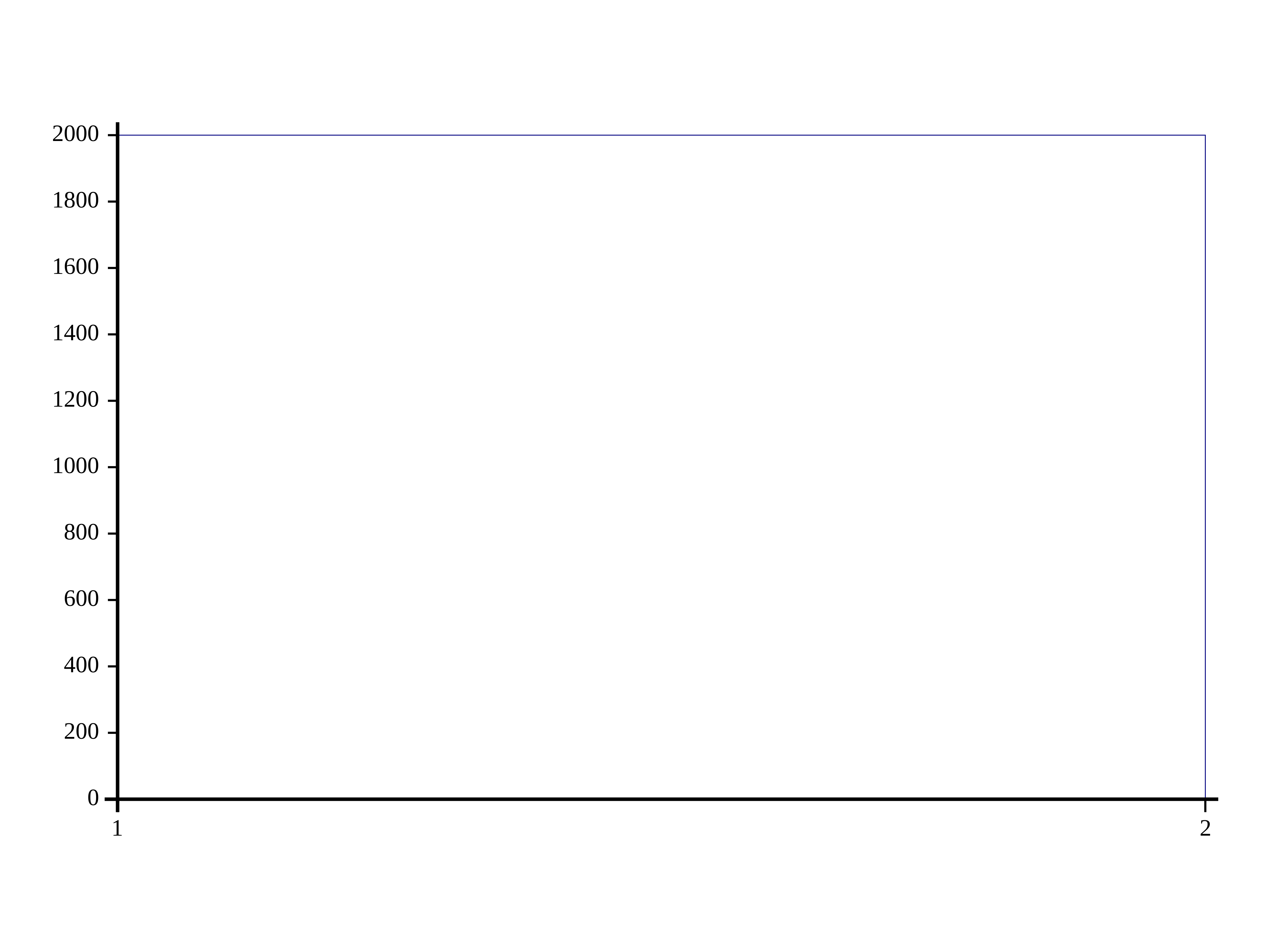
If the input is 1 we always get 1.
]plot -type=Histogram ? 2000 ⍴ 7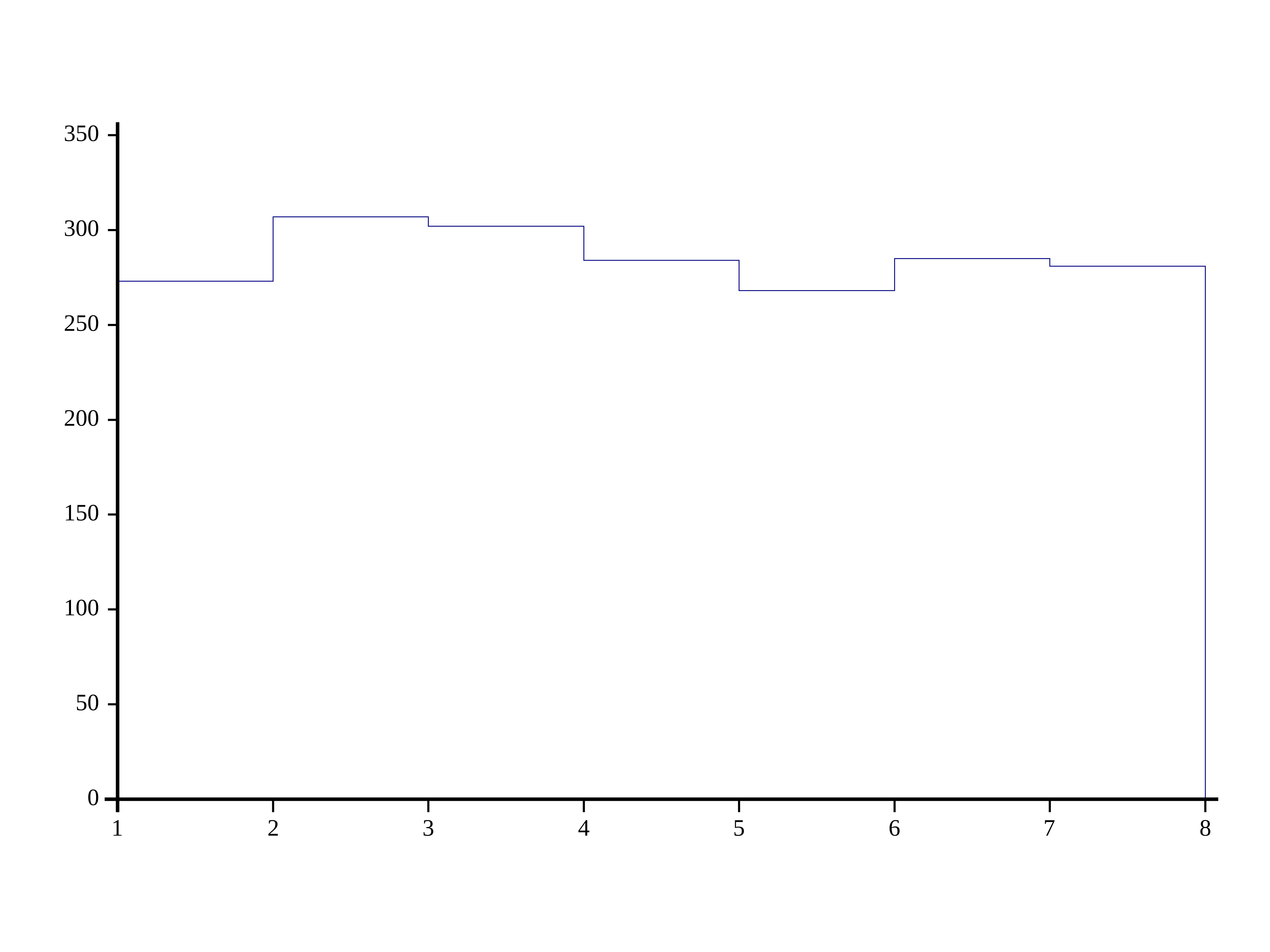
And here is a confirmation that we seem to get a uniform distribution over all the choices if we put an integer greater than 0 .
If we put a non-integer we get an error.
?0.5
DOMAIN ERROR: Roll right argument must consist of non-negative integer(s)
      ?0.5
      ∧
Dyadic use
If we use ? dyadically, we use a function called Deal.
And Deal gets us random permutation choosing k out of the n we had without replacement.
So 13 ? 52 will give us 13 numbers from ⍳52.
⎕ ← 'Length of result: ' (⍴97? 99)
97 ? 99
Length of result: 97 9 87 58 6 66 45 7 80 76 93 67 51 73 54 36 57 69 46 16 11 19 23 32 17 47 75 30 28 92 25 62 60 21 82 41 3 13 37 94 74 89 26 22 10 61 65 4 20 50 59 42 79 12 77 72 70 40 64 97 5 68 18 52 43 99 95 96 71 31 34 33 81 85 88 78 55 8 83 90 29 98 48 27 53 56 91 39 44 24 1 15 84 49 86 14 2 63
The above seems cool, but the only use-case that I could think of right now that you'd regularly use would be to shuffle some vector.
Since the first and second argument can be the same. So if we have a vector of length 99 and we want random indices we can do something like 99 ? 99, and get the shuffled indices.
99 ? 9951 65 96 8 20 87 56 1 62 84 30 6 46 83 21 24 74 63 67 5 14 73 4 81 36 15 68 40 41 86 10 98 25 2 69 91 71 49 95 53 34 11 72 61 9 23 76 79 13 32 52 7 3 55 88 37 89 50 44 77 82 38 39 80 18 92 28 78 17 94 57 19 58 35 33 64 90 43 16 29 48 27 54 45 60 12 22 47 97 85 66 59 42 75 31 26 93 99 70
I was also wondering if the second argument is a vector, if it would deal you X elements of the vector, since the function is called Deal.
w ← 1 2 4 8 16

3 ? w
LENGTH ERROR
      3?w
       ∧
But it doesn't. Which is fine because, you can get there easily anyways.
w[3?⍴w]16 2 4
Normal numbers
I was interested to see wether the normal distribution is implemented in dyalog, but it seems as though it isn't.
https://dfns.dyalog.com/n_contents.htm
I guess this was the page. I suspect its just a page where lots of good stuff is?? Anyways they have a NormRand and this is the implementation.
NormRand←{                          ⍝ Random numbers with a normal distribution
   depth←10*9                           ⍝ randomness depth - can be larger from v14.0
   (x y)←⊂[1+⍳⍴,⍵](?(2,⍵)⍴depth)÷depth  ⍝ two random variables within ]0;1]
   ((¯2×⍟x)*0.5)×1○○2×y                 ⍝ Box-Muller distribution
}

{+/⍵÷⍴⍵}¨NormRand¨10*⍳5
0.3337293743 0.0563430265 0.0231167616 ¯0.0006115008003 0.00111984966
To me this is actually pretty sick. According to Wikipedia this algorithm is kinda old (almost 100 years), but apparently pretty good on processors with vector units. (E.g. GPUs or modern CPUs). Since we are in APL its probably pretty good too.
The above code gets 10, 100, 1000, 10000, 100000 normal random numbers and takes their means. We would expect all of them to be quite close to 0 but the 100000 to be closest.
The above algorithm is pretty cool. I will try to do the interpretation
Box muller transform
d ← 10*9
w ← 20
⎕ ← 'Concat: ' (2,w)              ⍝ This part concats 2 and the input (the length we requested)
⎕ ← 'Output: ' ((2,w)⍴d)          ⍝ This makes a 2xw with entries d
⎕ ← '' (?((2, w)⍴d))÷d            ⍝ This takes 2xw random numbers between 1 and w and then divides them by d
 Concat:   2 20
 Output:   1000000000 1000000000 1000000000 1000000000 1000000000 1000000000 1000000000 1000000000 1000000000 1000000000 1000000000 1000000000 1000000000 1000000000 1000000000 1000000000 1000000000 1000000000 1000000000 1000000000
           1000000000 1000000000 1000000000 1000000000 1000000000 1000000000 1000000000 1000000000 1000000000 1000000000 1000000000 1000000000 1000000000 1000000000 1000000000 1000000000 1000000000 1000000000 1000000000 1000000000
   0.809071872 0.506960744 0.176644751 0.447176393 0.09769603  0.064839502 0.724852785 0.237949746 0.937169793 0.406416815 0.160212603 0.676102783 0.149541536 0.713072848 0.162178349 0.05294188  0.783331336 0.839000245 0.928971655 0.638300133
   0.139172256 0.726298137 0.313656287 0.366130325 0.578819883 0.243087457 0.543137433 0.731027775 0.885581504 0.603520226 0.777419555 0.695842502 0.976363713 0.465738575 0.456999316 0.261896563 0.296638724 0.666461724 0.301445244 0.136510824
w ← 2000
]plot -type=Histogram (?((2, w)⍴d))÷d            ⍝ This takes 2xw random numbers between 1 and w and then divides them by d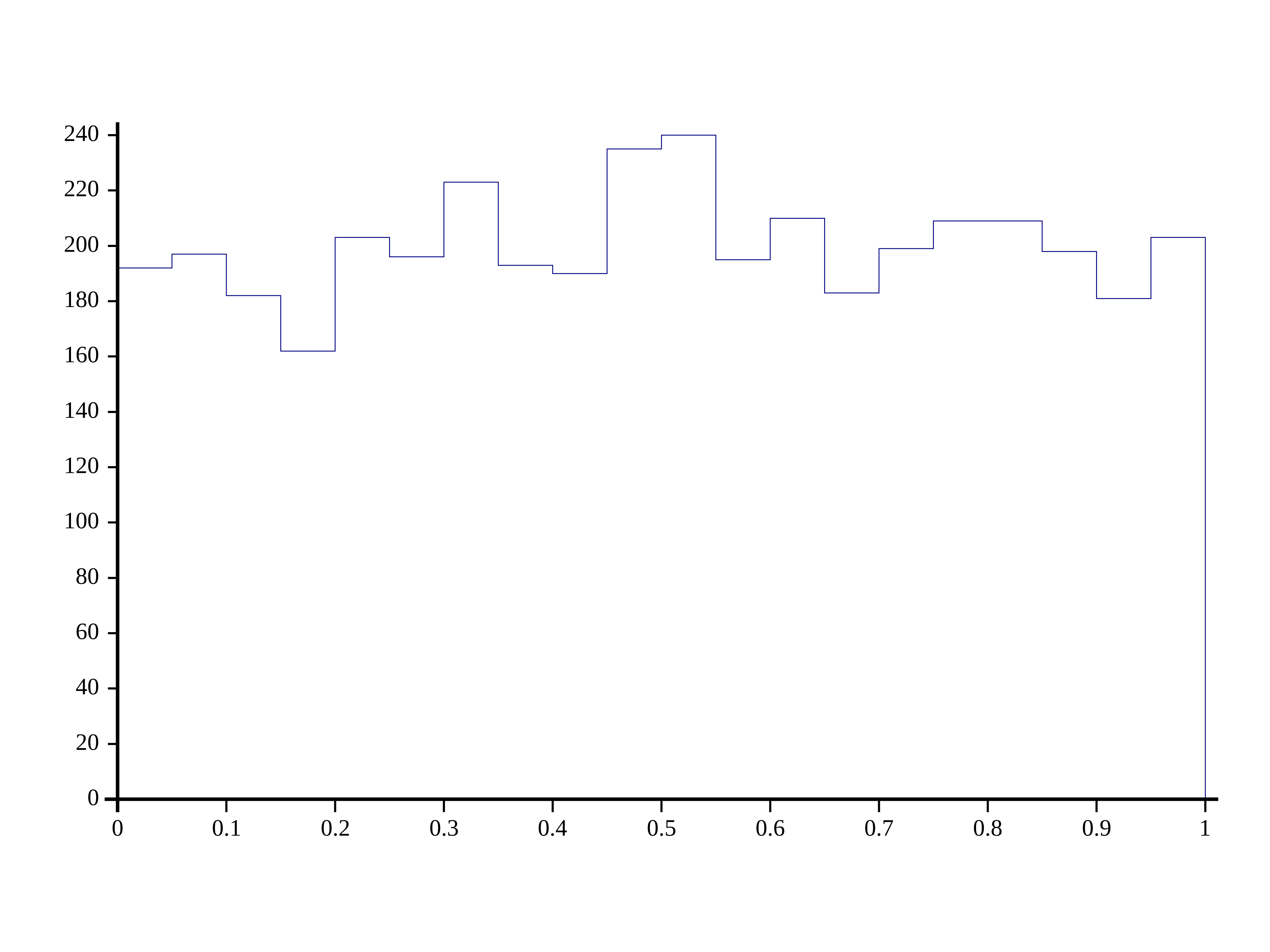
Oh, Ok, I think that this part just outputs uniform numbers between 0 and 1 no??
I bet this is a leftover from some other APL dialect / an older version of dyalog
that didn't have numbers a ?0 being random numbers between 0 and 1?
I think in this version of dyalog APL we just have this freely available with ?0
w ← 2000
]plot -type=Histogram ?(2, w)⍴0  ⍝ This takes 2xw random numbers between 0 and 1
Looking at the above plot, I think that it might just work. That means that the below should also probably work just as well to generate random numbers.
NormRand ← {                          ⍝ Random numbers with a normal distribution
   (x y)←⊂[1+⍳⍴,⍵]?(2,⍵)⍴0          ⍝ two random variables within ]0;1]
   ((¯2×⍟x)*0.5)×1○○2×y            ⍝ Box-Muller distribution
}

{+/⍵÷⍴⍵}¨NormRand¨10*⍳5
0.006324762607 ¯0.006668135531 ¯0.0153907865 0.0004685996237 ¯0.0002758807853
The means look good to me I guess.
]plot -type=Histogram NormRand 10000
And so does the histogram.
Moving on to the next part of the NormRand function. That part seems a bit harder to understand for me, because of two reasons, the first being just because I am not too used to APL programming in general, and the second reason is that the "Box-Muller" transform probably contains some interesting math?
The first part of the second line of the NormRand function that interested me was this Left shoe:
⊂ (Left shoe) (Written .z).
Apparently this is Enclose if used monadically and Partitioned Enclose if used dyadically.
I think that the brackets are gonna change what Monadic Enclose does. x and y are likely going to our pairs.
In pytorch lingo I guess we are using chunk and destructuring. ⍵ is the length we are expecting, that makes sense.
]help ⊂https://help.dyalog.com/19.0/Content/Language/Symbols/Left%20Shoe.htm
Running this we see that the random numbers are destructured, into two variables. Similar to maybe a tuple assignment in python.
(x y)←⊂[1+⍳⍴,w]?(2,w)⍴0
⎕ ← 'X: ' (x[⍳5]) '...'
⎕ ← 'Y: ' (y[⍳5]) '...'
X: 0.9565504493 0.2455306388 0.8781124073 0.5022757356 0.128598156 ... Y: 0.4688091298 0.5316777068 0.4411420703 0.3783071743 0.1422835975 ...
w ← 10 1
(x y)←⊂[1+⍳⍴,w]?(2,w)⍴0
⎕ ← 'Shape X:' (⍴ x) 'X: ' ( x[⍳4;1]) '...'
⎕ ← 'Shape Y:' (⍴ y) 'Y: ' ( y[⍳4;1]) '...'
Shape X: 10 1 X: 0.8144695925 0.2803614322 0.7332163463 0.0347636536 ... Shape Y: 10 1 Y: 0.1541552322 0.1200162438 0.6336035499 0.6484636464 ...
So the ⊂[1+⍳⍴,w] is basically clever indexing. Tbh, I don't quite understand why the , ravel has to be in there but .. lets just move on for now. This basically says, Enclose all axes except for the first, which is always 2. So that I can destructure.
Formula
Next up is the maths formula. Looks fun…
We can see some parts of the PDF in there. * means exponent so *0.5 is the square root. when used mondaically, The circle ○ is pi times. When used dyadically its the trig functions, and also the trig functions.
| ¯1 | Arcsin ⍵ |
| 1 | Sin ⍵ |
| -2 | Arccos ⍵ |
| 2 | Cosine ⍵ |
| 0 | (1-⍵*2)*0.5 |
((¯2×⍟x)*0.5)×1○○2×y ⍝ Box-Muller distribution0.5279529093 1.091826714 ¯0.5863436866 ¯2.082152329 ¯0.7987649983 ¯0.6489034688 1.17159251 0.3084765731 ¯0.3299759695 ¯0.7365224982
To me it looks like we are using it both dyadically and monadically here. First we do ○2×y which is pi * 2 * y I guess? And then we take the sine of that with 1○res. Thats the right half. The left half seems to be the square root of -2*pi*x. Nope, nevermind. That ⍟ Is actually called "Circle Star" and used monadically is the natural logarithm.
x0.8144695925 0.2803614322 0.7332163463 0.0347636536 0.3415325095 0.1137846227 0.5034192449 0.9348137478 0.9350711287 0.481514245
((¯2×⍟x)*0.5)0.6406530799 1.594788813 0.787800062 2.591981047 1.465818821 2.08492105 1.171607415 0.3671729012 0.3664223769 1.2089826
Ok, yeah I see what it does now. Its the root of the -2 log (x).
import numpy as np
[(np.log(.91337)*-2)**0.5
0.42570934471434346
Yeah this seems close enough.
((¯2×⍟x)*0.5)×1○○2×y ⍝ Box-Muller distribution¯0.6706356279 0.7126084526 0.8586799244 ¯0.04028840536 0.5791608201 ¯0.004212687272 ¯1.000324128 ¯0.2855864521 ¯0.09530046412 0.8951204028
So in "regular" math notation we are doing this:
\[ N_i = \sqrt{-2 \log(x_i) }\times \sin(2 \pi y_i) \]
TODO Yeah ok but why is this normal??
Anyways, we could also do some grid approximation with just this
Lets say we have a population of people. \( H \sim N(\mu, \sigma) \) Then we could roughly estimate the \( \mu, \sigma \) in the bayesian way, by making a grid out of all \( \mu, \sigma \), and look how likely each of these would have been to produce our dataset. To see that we would be roughly able to recover the original μ and σ , lets simulate a dataset of 400 people
(true_mu true_sigma) ← 165 5
data ← true_mu + true_sigma × NormRand(400)
]plot -type=histogram data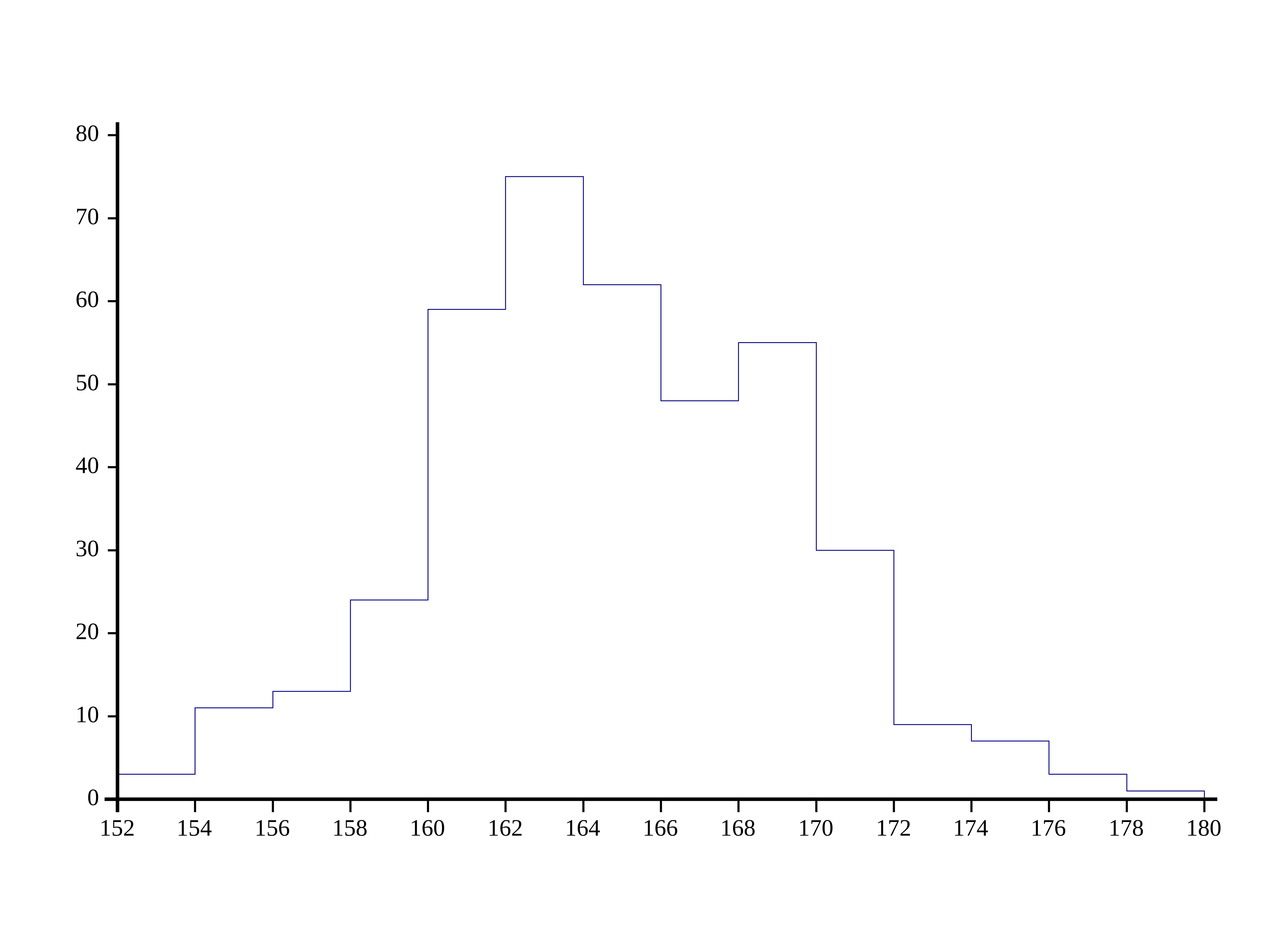
Here is the histogram of our simulated dataset.
Next, I want to make the PDF of Normal distribution.
I guess I would like a PDF of the normal distribution next?
\( N(x | \mu, \sigma) = \frac{1}{\sqrt{2 \pi \sigma^{2}}}e^{- \frac{ (x-\mu)^2 }{2\sigma^2} } \)
This is the PDF. not sure about the LHS tbh. I also tried doing it out of my head and got this:
\( N(x | \mu, \sigma) = \frac{1}{2 \sqrt{ \pi \sigma^{2}}}e^{- \frac{ x-\mu }{\sigma^2} } \) , which is not even close lol.
Anyways, lets start simple, and only do the PDF for a single value for now
s m x ← 1 0 2
prob ← (÷(○2×s*2)*.5)×*(-((x-m)*2)÷(2×s*2))

NormPDF ← {
    (s m x) ← ⍵
    (÷(○2×s*2)*.5)×*-((x-m)*2)÷2×s*2
}
w ← (1) (0) (2 1 0 ¯1 ¯2)

NormPDF w
0.05399096651 0.2419707245 0.3989422804 0.2419707245 0.05399096651
s m x ← ⊂[1](2 3 ⍴ 1 1 0 1 2 0)¯50+⍳100¯49 ¯48 ¯47 ¯46 ¯45 ¯44 ¯43 ¯42 ¯41 ¯40 ¯39 ¯38 ¯37 ¯36 ¯35 ¯34 ¯33 ¯32 ¯31 ¯30 ¯29 ¯28 ¯27 ¯26 ¯25 ¯24 ¯23 ¯22 ¯21 ¯20 ¯19 ¯18 ¯17 ¯16 ¯15 ¯14 ¯13 ¯12 ¯11 ¯10 ¯9 ¯8 ¯7 ¯6 ¯5 ¯4 ¯3 ¯2 ¯1 0 1 2 3 4 5 6 7 8 9 10 11 12 13 14 15 16 17 18 19 20 21 22 23 24 25 26 27 28 29 30 31 32 33 34 35 36 37 38 39 40 41 42 43 44 45 46 47 48 49 50
And we can plot it like htis
n ← 800

]plot (NormPDF 1 0 (¯4+0.01×⍳n))  (¯4+0.01×⍳n)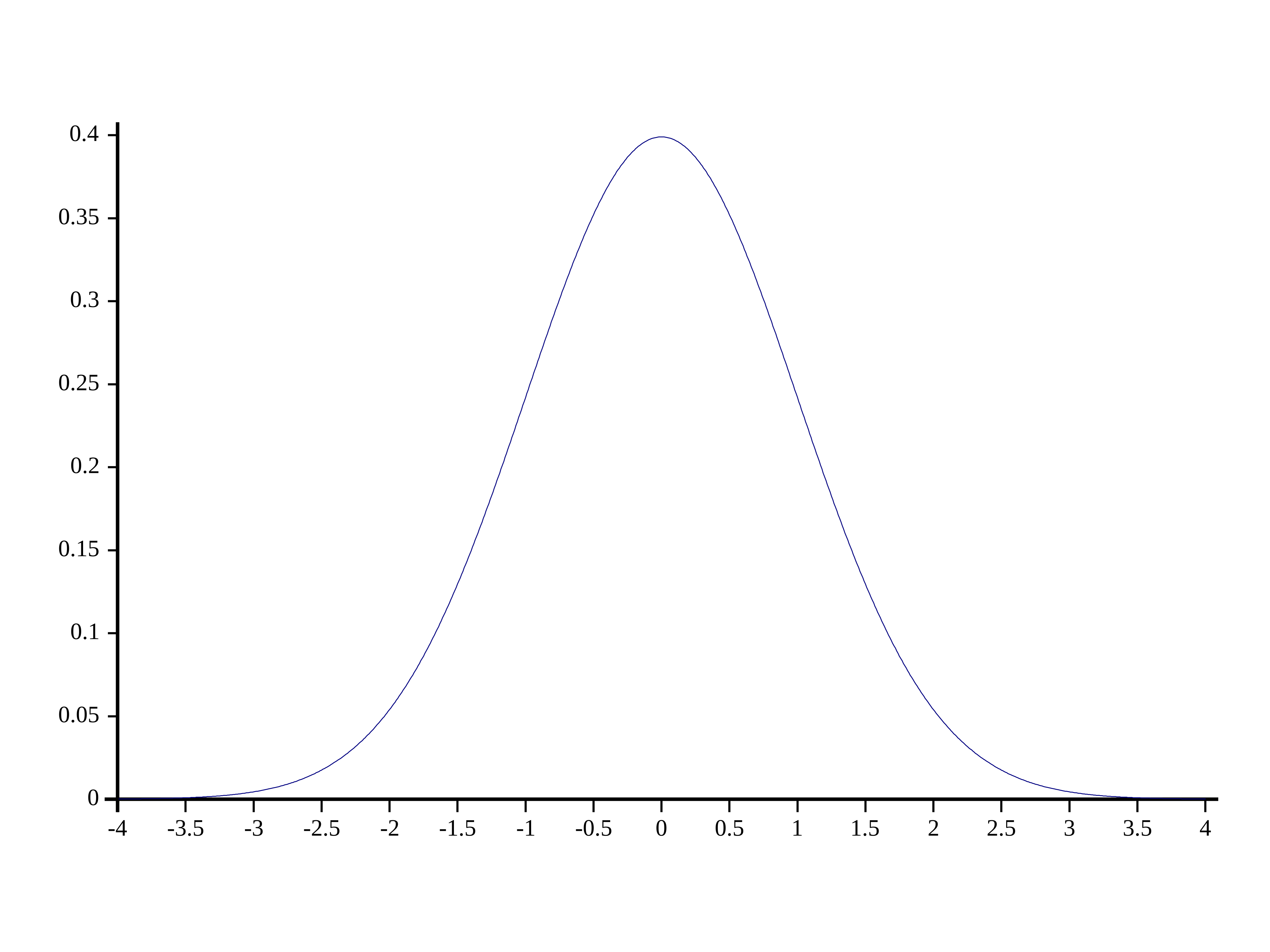
I also just remembered that you can turn on boxing like this:
]Boxing on
9(2 3)
⍴ 9(2 3)
⍴ ⊂9(2 3)
Was ON ┌─┬───┐ │9│2 3│ └─┴───┘ 2
To see more easily wahat is going on.